Storms, Prices, and the Power Grid
Storms, Prices, and the Power Grid
Predicting U.S. Power Outage Severity from Weather, Price, and Population Signals
by Arnav Goel and Paulina Pelayo (a2goel@ucsd.edu & ppelayo@ucsd.edu)
![]()
![]()
Rendered writeup: arnavgoel03.github.io/Power-grid-analysis Archived on Zenodo: 10.5281/zenodo.19707994 Course: DSC 80, The Practice and Application of Data Science, UC San Diego
Introduction
This project analyzes major U.S. power outages in the continental United States between 2000 and 2016, using a dataset compiled from the U.S. Department of Energy. A “major outage” is defined as an event that affects at least 50,000 customers or causes an unplanned firm load loss of at least 300 MW.
Our cleaned dataset contains 1,534 outages and 53 columns. We focus on:
OUTAGE.DURATION: total duration of the outage in minutes.CAUSE.CATEGORY: high level cause such as severe weather, equipment failure, or intentional attack.CUSTOMERS.AFFECTED: number of customers impacted.POPDEN_URBAN: urban population density.RES.PRICE: average residential electricity price by state.- Climate and seasonal fields such as
MONTH,CLIMATE.REGION, andANOMALY.LEVEL.
Our central question is:
How do weather conditions, electricity prices, and population density relate to the severity of major power outages, measured by outage duration?
Understanding how weather, electricity prices, and population density connect to outage duration helps utilities and policy makers predict where long outages are most likely, stage crews earlier, and invest in grid hardening where it actually matters.
This is getting more urgent as AI ramps up electricity demand through data centers and constant compute. A grid under heavier, more continuous load has less slack when storms hit, so failures can last longer and affect more people. Studying what drives outage severity is basically planning for a future where both climate stress and computing demand keep rising.
Data Cleaning and Exploratory Data Analysis
We performed several data cleaning steps to make the outage records usable for analysis:
- Combined separate date and time columns into full timestamps
OUTAGE.STARTandOUTAGE.RESTORATION, which makes time based comparisons consistent and lets us validate duration logic before doing any EDA or modeling. - Dropped impossible records where the restoration time was earlier than the start time, preventing negative or corrupted
OUTAGE.DURATIONvalues from skewing the ECDF and inflating error in downstream models. - Treated zeros in
CUSTOMERS.AFFECTED,OUTAGE.DURATION, andDEMAND.LOSS.MWas missing values since “0” in this dataset typically reflects “not recorded” rather than a true zero, which avoids biasing distributions and keeps missingness analysis meaningful. - Removed unused identifier columns such as
OBSandvariables, reducing noise and preventing models from learning patterns tied to row identifiers instead of real outage drivers.
To understand the distribution of outage duration, we first plotted an ECDF:
Roughly 80 percent of outages last fewer than about 3,000 minutes, so the distribution is heavily right skewed with a small number of extremely long events.
We also examined what actually causes outages. The bar chart below summarizes the frequency of high level causes:
Severe weather is by far the most common cause of major outages, followed by intentional attacks and system operability disruptions. Fuel supply emergencies are rare but, as we will see, they tend to be extremely long.
To study how outages relate to state level characteristics, we aggregated by state and looked at the relationship between urban density and outage count:
States with higher urban population density generally experience more major outages, although there is substantial variability across states. Dense infrastructure seems to go hand in hand with more frequent large outages.
Finally, we explored how outage size and duration relate:
Outages that affect more customers tend to last longer on average, but there is wide scatter. Even outages with similar customer impact can have very different durations, which suggests that other drivers such as cause and weather strongly influence recovery time.
To better compare the severity of different causes, we summarized outage duration by CAUSE.CATEGORY:
Fuel supply emergencies have the longest average and median outage durations, indicating rare but extremely severe events. Severe weather is the most common cause and also produces long outages. Intentional attacks and islanding tend to be shorter disruptions on average.
This shows strong seasonal effects on outage duration. Severe weather leads to long outages across all seasons. Fuel supply emergencies are most severe in winter, likely due to heating demands and constrained energy supply. Summer shows higher durations for operability failure, possibly from increased use of air conditioning and peak electricity usage.
Comparing outage duration across price groups shows that low price states experience longer typical outages than high price states, with both higher mean and median durations. This suggests that electricity pricing may serve as a proxy for infrastructure investment and grid reliability, motivating a formal hypothesis test of whether high price states systematically experience shorter outages.
Assessment of Missingness
We focused our missingness analysis on DEMAND.LOSS.MW, the estimated megawatt load that could not be served during an outage.
NMAR reasoning
The missingness of DEMAND.LOSS.MW is plausibly Not Missing At Random (NMAR). In very large or chaotic outages the monitoring infrastructure itself may be damaged or overloaded, which makes it harder to measure demand loss accurately. Very small outages might not warrant a formal MW estimate at all. Since the chance that demand loss is recorded likely depends on the true but unobserved size of the outage, we cannot fully explain missingness using other observed columns alone.
Dependency on observed columns
We then asked whether the missingness of DEMAND.LOSS.MW depends on particular observed features.
- Dependency on outage cause
We created an indicator column LOSS_MISSING for whether DEMAND.LOSS.MW is missing and compared missingness rates across CAUSE.CATEGORY using a permutation test. The observed difference between the highest and lowest missingness rate across causes was much larger than in the null distribution, giving a p value near 0. This suggests that missingness does depend on the cause of the outage.
We visualized this using a bar chart of missingness by cause:
- Dependency on month
Next we tested whether missingness depends on MONTH. Our test statistic was the difference in mean month between rows where DEMAND.LOSS.MW is missing and rows where it is observed. A permutation test yielded a p value around 0.23, so we do not find evidence that missingness depends on month.
This is also reflected in the box plot below:
Permutation tests show that the missingness of DEMAND.LOSS.MW depends strongly on CAUSE.CATEGORY (p ≈ 0), indicating that missingness is not purely random and is related to observed outage characteristics. In contrast, missingness does not appear to depend on MONTH (p ≈ 0.23), suggesting no seasonal reporting bias. Therefore, the missingness mechanism is consistent with MAR with respect to outage cause, while remaining potentially NMAR with respect to the true unobserved magnitude of power lost.
Hypothesis Testing
Motivated by our economic analysis, we tested whether states with higher residential electricity prices tend to experience shorter outages.
- Null hypothesis (H₀): The distribution of outage durations in high price states is the same as or stochastically greater than in low price states.
- Alternative hypothesis (H₁): Outage durations in high price states are stochastically smaller than in low price states.
We split states into “High Price” and “Low Price” groups using the median of RES.PRICE and compared their outage duration distributions using a one sided KS style statistic. The statistic measures how often the ECDF of the high price group lies above the ECDF of the low price group.
A permutation test with 1,000 random label shuffles produced a p value of about 0.007. At a significance level of α = 0.05 we reject the null hypothesis. The evidence suggests that states with higher residential prices tend to have shorter outage durations than states with lower prices, which is consistent with the idea that higher prices may be associated with greater investment in grid reliability.
Justification for the design choices:
- High vs Low Price split at the median of
RES.PRICE: Creates two balanced groups without an arbitrary cutoff, making it easy to compare outage durations between higher priced and lower priced states. - Permutation test: Outage durations are highly right skewed, so a nonparametric shuffle test avoids normality assumptions and directly checks whether the observed difference could occur by chance.
- One sided ECDF / KS style statistic: Matches our directional question (“are high price states shorter?”) and compares the full distributions rather than just the mean, which can be dominated by extreme outages.
- Significance level α = 0.05: A standard threshold that provides a reasonable balance between false positives and false negatives for this context.
Framing a Prediction Problem
We next turned our descriptive findings into a prediction task.
- Prediction problem: Predict the duration of a major power outage in minutes.
- Problem type: Regression.
- Response variable:
OUTAGE.DURATION.
Predicting outage duration matters because it gives utilities a way to estimate restoration timelines, triage scarce crews, and communicate expectations to customers and emergency services.
- Evaluation metrics: Root Mean Squared Error (RMSE) and R².
- RMSE: We use RMSE because it measures prediction error in the same units as the target (minutes), which makes it directly interpretable for outage planning. RMSE also penalizes large mistakes more than MAE, which matters here since severely underestimating a long outage is more costly than being slightly off on a short outage.
- R²: We include R² to summarize how much variation in outage duration our features explain compared to a simple baseline (predicting the mean). This helps contextualize RMSE, since an RMSE value alone can be hard to judge without knowing how predictable the outcome is overall.
At the time of prediction we assume we know where and when the outage occurs plus high level information about the event, such as its cause, but not its eventual duration. Features we consider include:
- Geographic and climate features:
U.S._STATE,CLIMATE.REGION,CLIMATE.CATEGORY,MONTH. - Demographic features:
POPDEN_URBAN,POPULATION. - Economic features:
RES.PRICE,COM.PRICE,IND.PRICE. - Event level features:
CAUSE.CATEGORY.
Baseline Model
We start with a Linear Regression baseline because it is simple, fast to train, and easy to interpret. As a baseline, it gives us a clear “minimum bar” for performance, and it helps us see whether our features contain any usable signal before moving to more flexible models.
In this baseline, we assume outage duration can be approximated as a linear combination of our features plus noise. Formally, the model is:
\[\hat{y} = \beta_0 + \beta_1 x_1 + \beta_2 x_2 + \cdots + \beta_p x_p,\]where (y) is OUTAGE.DURATION, the x_i are the (preprocessed) features, and the beta_i coefficients are learned from the training data by minimizing squared error:
This setup provides a transparent baseline because each coefficient represents the average change in predicted outage duration associated with a one unit change in a feature (holding others fixed), after standardization and one hot encoding.
We restricted the baseline to a small but meaningful feature set to avoid overfitting and to keep the model aligned with what would realistically be known early in an outage: a proxy for local demand and urbanization (POPDEN_URBAN), an economic proxy for grid investment and structure (RES.PRICE), the type of event (CAUSE.CATEGORY), and seasonality effects (MONTH).
Our feature set:
POPDEN_URBANRES.PRICECAUSE.CATEGORYMONTH
Additionally, we dropped rows where OUTAGE.DURATION is missing.
To make the model usable on messy real data, we fit everything inside a single scikit-learn Pipeline with a ColumnTransformer:
- Numerical (quantitative) features (
POPDEN_URBAN,RES.PRICE,MONTH):- Imputed with the median to handle missing values robustly.
- Standardized with
StandardScalerso that the regression coefficients are on a comparable scale.
- Categorical features (
CAUSE.CATEGORY):- Nominal feature.
- Imputed with the most frequent category.
- One hot encoded so that the model can learn different baseline duration shifts for each cause type.
We evaluated this model on a held out test set.
- Baseline RMSE: about 6,404 minutes.
- Baseline R²: about 0.165.
This indicates modest predictive ability, as the model explains about 16.5 percent of the total variation in outage duration and makes relatively large prediction errors in absolute time. Thus, the model captures some signal but leaves most of the variation in outage duration unexplained, which motivated us to engineer additional features and move to a more flexible model.
Final Model
Features added and why they make sense (data generating process)
To better reflect how outages happen and get resolved, we added two features:
-
IS_WEATHER(severe weather indicator). Severe weather outages are driven by a different failure and recovery process than non weather outages. Storms can cause widespread, simultaneous damage across a region, which can delay restoration due to limited crews, blocked access, and cascading infrastructure impacts. Encoding this as a binary feature helps the model separate weather driven outages from other causes instead of forcing one “average” relationship across all events. -
LOG_POPDEN= log1p(POPDEN_URBAN). Urban density is highly skewed, and its effect on restoration is plausibly nonlinear. Moving from low to medium density can change outage logistics a lot, but going from already dense to extremely dense areas may have diminishing returns. Takinglog1preduces the influence of extreme values and better matches this “diminishing returns” structure.
Our final feature set was: LOG_POPDEN, IS_WEATHER, RES.PRICE, MONTH, and CAUSE.CATEGORY.
Modeling algorithm and how we selected hyperparameters
We used a RandomForestRegressor because outage duration depends on nonlinear interactions (for example, the effect of a cause can differ by month or weather conditions), and random forests can capture these patterns without requiring us to manually specify them.
We kept the same train/test split and used a single scikit-learn Pipeline:
- Numeric features: median imputation.
CAUSE.CATEGORY: most frequent imputation plus one hot encoding.- Model:
RandomForestRegressor.
To select the final Random Forest, we used GridSearchCV (5 fold CV) over the following hyperparameters (tree depth, estimators, etc.):
n_estimators∈ {100, 200}.max_depth∈ {None, 10, 20}.min_samples_leaf∈ {1, 5}.
The best performing model used n_estimators = 200, max_depth = None, and min_samples_leaf = 5.
We chose the best setting based on cross validated performance (negative RMSE), then evaluated that best model once on the held out test set.
Performance and improvement over baseline
On the held out test set, the final model achieved:
- Final RMSE: about 6,189 minutes.
- Final R²: about 0.220.
Compared to the baseline (RMSE about 6,404; R² about 0.165), this improves RMSE by about 200 minutes and increases explained variance by several percentage points. This is consistent with the added features helping the model better separate weather driven dynamics and handle the nonlinear effect of density, while the random forest captures interactions the linear baseline cannot.
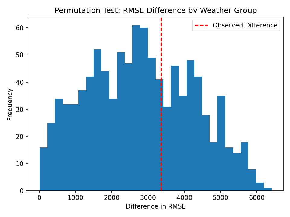
Fairness Analysis
We used a permutation based fairness test to check whether our final Random Forest model performs differently on severe weather vs non weather outages, using RMSE on the test set.
- Groups (using
IS_WEATHER):- Group X: severe weather outages (
IS_WEATHER = 1). - Group Y: non weather outages (
IS_WEATHER = 0).
- Group X: severe weather outages (
-
Metric: RMSE (computed separately for each group).
-
Test statistic: absolute difference in RMSE. \(T = \left| \mathrm{RMSE}_{\mathrm{weather}} - \mathrm{RMSE}_{\mathrm{non\ weather}} \right|\)
-
Significance level: α = 0.05.
- Hypotheses:
- Null hypothesis (H₀): The model’s RMSE is the same for severe weather and non weather outages.
- Alternative hypothesis (H₁): The model’s RMSE differs between severe weather and non weather outages.
- Procedure:
- Compute RMSE for Group X and Group Y on the test set.
- Shuffle the group labels (
IS_WEATHER) 1,000 times, keeping predictions fixed. - Recompute (T) each time to form the null distribution.
- The p value is the fraction of shuffled (T) values at least as large as the observed (T).
- Result: The permutation test produced p ≈ 0.366, so at α = 0.05 we fail to reject the null hypothesis (H₀). The results do not provide sufficient statistical evidence that the model performs differently for severe weather outages than for non weather outages. Therefore, we do not find the model to perform unfairly under this metric.
Repository Layout
.
├── README.md                 Full writeup (this file), rendered at the site above.
├── index.md                  Jekyll entry point for the rendered site.
├── _config.yml               Jekyll and Hydejack theme configuration.
├── CITATION.cff              Machine readable citation for Zenodo, GitHub, and academic tools.
├── LICENSE                   MIT.
├── image1.jpg                Cover image for the rendered site.
└── assets/                   Interactive Plotly HTML figures and tables embedded in the writeup.
How to Cite
If you reference this work, please cite the Zenodo record so the citation resolves to an immutable snapshot:
Goel, A., & Pelayo, P. (2026). Power Grid Outage Analysis: Predicting U.S. Outage Severity from Weather, Price, and Population Signals (v1.0.0). Zenodo. https://doi.org/10.5281/zenodo.19707994
A machine readable citation is provided in CITATION.cff. On GitHub the “Cite this repository” button will render this automatically.
This project was completed for DSC 80: The Practice and Application of Data Science at UC San Diego.